



Price elasticity of demand is one of the most useful ideas for finding the right price for a product, and one of the hardest to calculate reliably. In theory, elasticity tells us how demand responds to price changes. In practice, observed demand is shaped by many forces at once: promotions, seasonality, stock availability, competitor moves, lifecycle effects, and ordinary imperfections in retail data.
In this article we present a novel methodology for estimating product-level price elasticities, built for the messy conditions of real-world retail, where price changes are sparse, demand is noisy, and clean experiments are rarely available. Its central idea is that elasticity estimation is better approached as a two-stage problem.
In the first stage, a predictive layer extracts a broader and more usable demand signal from sparse, noisy, and uneven product-level data. In the second stage, that signal is translated into a demand model that can support price optimization rather than simply describe price sensitivity after the fact.
The difference is what makes the approach work in production. The demand curve used in live pricing must be strong enough to support decisions under real commercial conditions, and that means treating price as only one input among several. The system also needs to understand the conditions in which each price was observed.
A more fundamental obstacle is that many products do not change price often enough, or in conditions that isolate the price effect, to support reliable direct estimation on their own. An approach that depends only on one-step product-level fitting tends to deliver either narrow coverage or fragile results. The two-stage design avoids that trap: it expands the usable demand signal first, then turns that signal into an optimization-ready demand curve.
The sections that follow explain elasticity in practical terms, outline the principles behind the two-stage approach, and show why a modern elasticity framework must be both scientifically grounded and commercially usable.
Why elasticity matters in real pricing work
Every pricing decision contains an implicit assumption about customer response. When a retailer raises price, lowers price, or holds steady as market conditions change, they are making a demand forecast whether they say so or not.
Elasticity makes that assumption explicit.
At a practical level, elasticity helps pricing teams answer questions such as:
- Which products can tolerate a price increase with limited volume risk?
- Which products are highly price-sensitive and need tighter competitive positioning?
- Where is discounting likely to create incremental demand, and where does it mostly give away margin?
- Which categories behave consistently enough for automation, and which need human review?
For pricing professionals, the value of elasticity is not in elegant theory alone. It lies in improving decisions under uncertainty, and in turning observed demand response into a demand curve solid enough to support price optimization.
What elasticity means
Elasticity measures the relationship between a percentage change in price and the resulting percentage change in demand. Formally, it is the ratio of the two:
where %ΔQ is the percentage change in demand and %ΔP is the percentage change in price.
A product with an elasticity of -2, for example, sees demand fall by roughly 2% for every 1% price increase. The value is almost always negative, since demand and price usually move in opposite directions, so what matters is how far below zero it sits. Products more sensitive than -1 are considered elastic: demand reacts more than proportionally to price. Products between -1 and 0 are inelastic: demand moves less than the price change that caused it.
This is a powerful concept, but it is easy to oversimplify. An observed change in demand is not automatically a pure price response. The definition above assumes that everything other than price is held fixed, which rarely holds in raw retail data: promotions, seasonality, stock, and competitor moves shift demand at the same time price changes. A credible elasticity system therefore has to ask a harder question: how much of the movement should be attributed to price, and how much belongs to the surrounding commercial context?
Elasticity is also more than a descriptive metric. In practice, it is derived from a demand curve, an operational view of how volume is likely to move across a range of possible prices. That curve is what lets pricing teams compare the expected effect of different price points on revenue, margin, and business goals. Elasticity summarizes the curve at a reference price, but the curve itself is what drives optimization. That is the bridge from diagnosis to action: the curve captures how volume moves across a range of prices, and elasticity makes that sensitivity actionable at a single reference point.
The next two figures make the same practical point from two angles: raw price-sales patterns can be inspected directly, but they should not be treated naively as causal price response when calculating elasticity. Figure 1 shows how seasonality can change the apparent relationship between price and demand. Figure 2 shows how stock constraints can distort both observed sales and the price signal. Promotions, competitor moves, lifecycle effects, assortment changes, and other commercial conditions can create similar distortions, which is why raw price-sales observations should be treated as signals to validate rather than clean experiments.
Example products: three monthly contexts
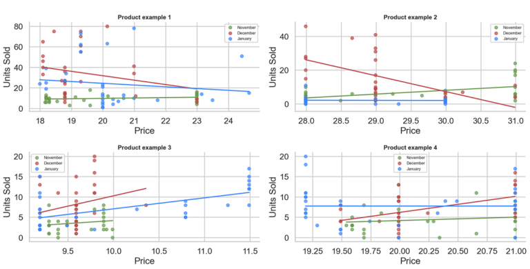
Figure 1. Four example products illustrate that context matters alongside price. Different months show different price ranges, sales levels, and apparent price-demand relationships, and in several cases demand even rises with price. That upward slope is not a sign that higher prices lift sales; it reflects confounders such as seasonal demand or competitor moves that coincide with price changes. A positive slope can therefore be acceptable in this diagnostic view precisely because the plot is not a controlled price experiment. The naive regression lines make the point that raw price-sales slopes can mislead when context is ignored, which is why elasticity cannot be read directly off observed data.
When stock runs low, both sales and the price signal become unreliable
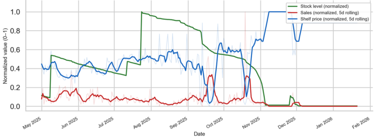
Figure 2. A real product from a live retail assortment, anonymized. All three series are normalized to the same 0-1 scale for comparability. From May through October the product is well-stocked and sells steadily. From November onward, as stock falls toward zero, sales collapse and the shelf price is pushed up, likely a deliberate move to suppress demand on a product that can no longer be supplied. During this period the posted price reflects a stock-rationing decision, not normal demand generation, so both signals become unreliable for elasticity estimation. Observations like these are excluded from the model.
The practical challenge
Pricing optimization at scale calls for a robust framework that can support tens of thousands of products across changing market conditions. This creates several practical requirements:
- Coverage: the system must yield results for a large share of the assortment, not just the products with the cleanest data.
- Stability: outputs should not swing wildly because of temporary noise.
- Interpretability: analysts need to understand why an estimate can be trusted.
- Operational fit: the methodology must support live pricing decisions, not just retrospective analysis.
- Guardrails: when product-level support is weak, the system should degrade gracefully rather than produce false precision.
This is where many elasticity estimation methods struggle. A model may look statistically impressive on a subset of clean products yet still fail to serve the broader pricing process.
The core tradeoff: specificity vs. reliability
One of the central challenges in elasticity work is that the most stable and intuitive analytical unit is often broader than the individual product. Category-level patterns are easier to interpret and usually more statistically reliable. Yet pricing decisions ultimately need to be made at the product level, where the recommendation becomes actionable.
That creates a practical tension. Category-level estimates can be reliable but too coarse for product-level optimization. Product-level estimates are more actionable, but many products do not change price often enough, or do not have enough clean history, to estimate a reliable response in isolation. In those cases, the usable demand signal for a single product can be much smaller than its transaction history first suggests.
This is why grouping and generalization are not shortcuts. They are a necessary part of building a usable elasticity system.
The task, then, is not to choose between product-level modeling and grouping as if one were always better. It is to work at the most specific level the data can support, and to generalize carefully when it cannot. A credible elasticity methodology must manage that tradeoff explicitly.
A practical two-stage methodology
A practical elasticity methodology of this kind is built around a central insight: the demand curve is not a fixed property of a product: it is a context-specific object. The same product in peak season versus the off-season, or facing an aggressive competitor versus a quiet market, will produce a different demand curve even if its underlying price sensitivity has not changed. Elasticity is always computed at a reference price within a reference context. When that context changes, the methodology re-estimates from the updated commercial state.
This has a practical consequence for how the methodology is structured. The predictive layer does not ask “what would sales be at this price?” in the abstract. It asks: given a relevant reference context for this product, the time of year, the price trajectory, the competitive landscape, and the commercial scenario being evaluated, what would sales be if we changed only the price?
To answer this, stage 1 trains a predictive model on the product’s historical data and uses it to produce a context-specific demand signal: holding the chosen reference context fixed, it samples demand across the product’s observed price range. In live repricing, that reference context is often the current commercial state; in simulation, it may be another scenario the business wants to evaluate. Stage 2 then fits a parametric demand curve to that signal, selecting the most appropriate functional form from a set of candidate models, which matters when demand profiles vary as much as they do across a real retail assortment. The result is an analytical demand curve grounded in the relevant commercial reality, more useful for optimization than a plain price-versus-sales regression.
The logic, in short: rather than assume every product can be modeled directly, cleanly, and independently, the methodology first expands the usable demand signal and only then fits a demand model suitable for pricing decisions, maximizing useful coverage while preserving credibility.
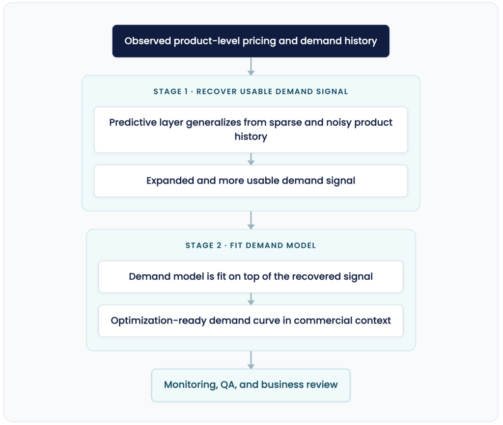
Figure 3. The two-stage logic of the methodology: first recover a usable demand signal from sparse product history, then fit a demand model that can support optimization.
Example Product Paths from Observed Data to Fitted Demand Curves
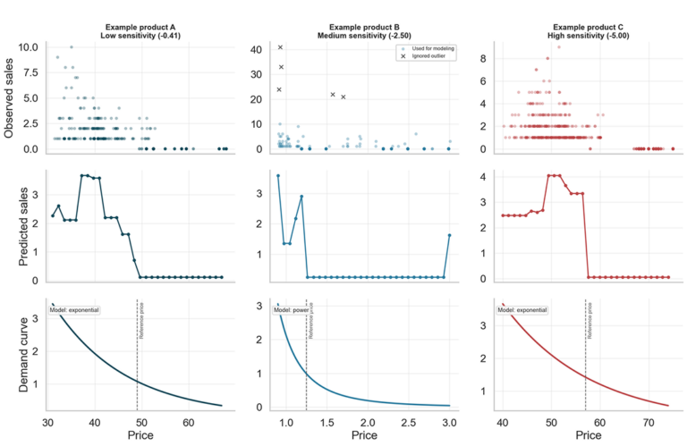
Figure 4. The two-stage methodology applied to three real products spanning low, medium, and high price sensitivity. Each column follows one product through the full pipeline. The top row shows raw observed sales plotted against price, spanning all observed commercial contexts across the product’s history. The middle row shows stage 1 output: the predictive layer holds a chosen reference context fixed and samples demand at prices across the observed range. These plots are a projection of the full model view: seasonality, competitor prices, and other contextual features that the predictor uses are collapsed into a two-dimensional price-versus-units chart, which is why the predicted signal may look different from the raw scatter above. The bottom row shows stage 2 output: a parametric demand curve fitted to that context-specific signal. The vertical dashed line marks the reference price at which the elasticity value shown in each panel title is evaluated. A different reference price, or a different commercial context, would produce a different curve and a different elasticity value.
At a high level, the approach follows four principles.
1. Start with observable commercial reality
The foundation is transactional and pricing data that reflects actual market behavior over time. The methodology is designed to learn from observed responses in live retail conditions rather than from idealized assumptions.
This matters because pricing teams need estimates that remain useful across real categories, markets, and customer contexts.
2. Separate signal from distortion
Not every observed volume change is equally informative about elasticity. A practical methodology must judge which observations carry useful price signal and which should be down-weighted before drawing conclusions.
This is one of the most important differences between a pricing-grade system and a simplistic price-response calculation.
Certain price points act as psychological thresholds for shoppers: a price move that crosses one can affect demand differently from an equal-sized move that does not. To reflect this, our methodology does not read prices in raw form alone. It first snaps price into psychologically anchored buckets, with finer increments at low price points and coarser increments at higher ones, so that a move crossing a bucket boundary registers as a distinct price event. A shift from $9.99 to just above $10 registers as a genuine price change, while a one-cent drift within a bucket does not. Reading price this way keeps the model from treating a threshold crossing and an ordinary in-bucket move as the same event.
3. Use the most specific supported granularity
The methodology applies a quality-driven cascade to determine which stage 1 predictor is used for each product.
For well-supported products, those with sufficient history and price variation, the methodology first tries a product-level predictor built from the product’s own data. If that predictor lacks sufficient confidence, or if the resulting demand curve does not meet the fit-quality threshold, the product falls back to a group predictor, though its own data still contributes to building that group model. In either case, stage 2 fits an individual demand curve.
Products with very sparse data present a different challenge: their history is too thin to serve even as a reliable product-level predictor. For these products, the methodology uses a clustering logic we refer to as propagation: assigning each sparse-history product to the most suitable modeled group based on product properties such as commercial segment (key value items, sales drivers, or profit generators), product categories, price level, and sales volume. The group model then produces a demand signal for that product while still using its own commercial context, its prices, competitive dynamics, and seasonal pattern, in stage 1. Stage 2 then fits an individual demand curve, so the product remains individually optimizable despite its sparse history.
When a retailer’s overall data is limited, some sparse-history products may not have a sufficiently reliable group match available. In those cases, maintaining broad coverage requires a conservative fallback rather than leaving the product unserved.
The key principle is to use the most specific predictor the data can credibly support, and to widen the usable signal through prediction before fitting an optimization-ready demand model.
4. Prefer robustness over false precision
In production pricing, a slightly less precise estimate that is stable, explainable, and decision-safe is often more valuable than a mathematically elegant estimate that is fragile.
This is especially true when the output is used by merchandisers, pricing managers, and commercial leaders who need confidence, not just coefficients.
Robustness also requires quality thresholds. If the predictive stage is not accurate enough, or if the fitted demand model does not explain the observed pattern well enough, the methodology should fall back to a more conservative level rather than overstate confidence.
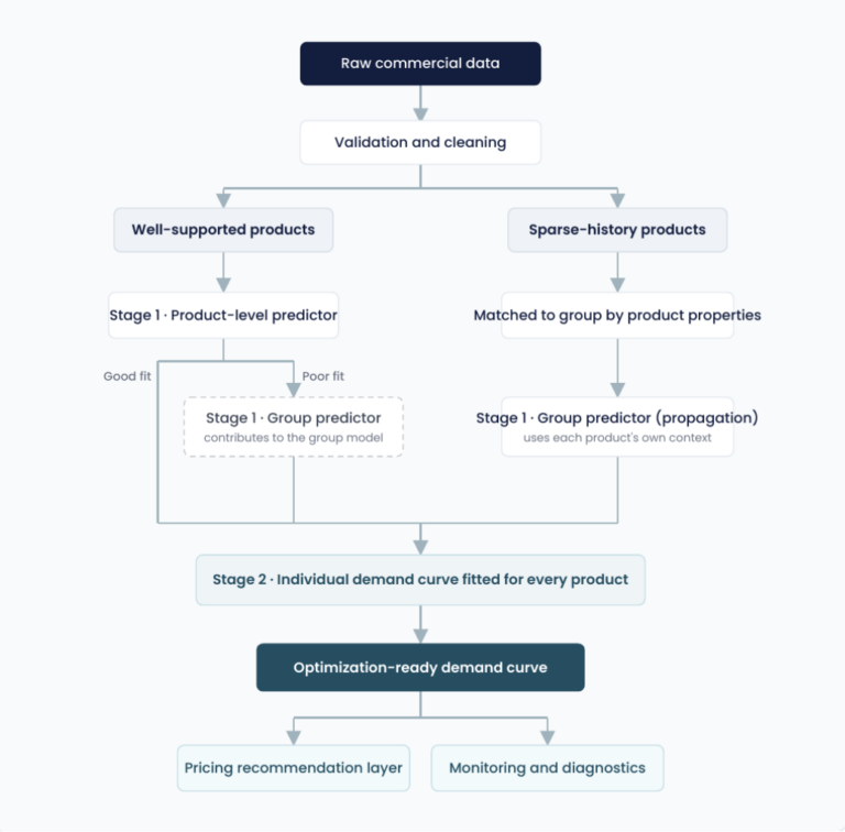
Figure 5. The production pipeline from raw data to pricing output. Products with sufficient history first try a product-level predictor in stage 1. If confidence or fit quality is too weak, the product moves to a group predictor while still contributing to that group model. Sparse-history products take the propagation path: they are matched to a suitable group by product properties, and the group predictor uses each product’s individual commercial context to produce its demand signal. All paths converge at stage 2, where an individual demand curve is fitted for every product regardless of which predictor was used. The output feeds both the pricing recommendation layer and continuous monitoring.
Monitoring the system in production
A production elasticity system should be monitored like a pricing decision engine, not treated as a one-time model run. The key question is not only whether a model produced an output, but whether the system is still operating at the same level of evidence and reliability as before.
Useful monitoring should track both coverage and quality: how much of the assortment and revenue are covered, how many products are modeled directly versus through group or propagation logic, how often fallback is used, and whether confidence, fit quality, or rejection rates are changing over time. It should also watch upstream data-health signals such as missing days, stock constraints, price variation, catalog changes, and competitor-data availability.
Together, these indicators create an early warning layer. If product-level coverage suddenly falls, propagation rises, or fallback usage spikes, the business can investigate upstream data drift, catalog changes, stock problems, or pipeline issues before the change appears as poor pricing behavior. Monitoring also gives pricing teams a practical governance view: which recommendations are ready for automation, which should be reviewed, and which are supported only by conservative fallback logic.
Granularity Distribution Over Time
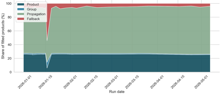
Figure 6. Drawn from a live retail assortment, anonymized. Each product is assigned to one of four modeling levels (product, group, propagation, or fallback) depending on data quality and coverage. Product means the demand signal is recovered from the product’s own history. Group is used when product-level support is weaker but the product can still contribute to a broader model. Propagation is used for sparse-history products that are assigned to a matching group by product properties. Fallback is reserved for products that cannot be matched to a suitable modeled group. The temporary degradation in mid-January illustrates why monitoring matters: data or code issues can surface as unexpected shifts in the granularity mix, and a well-designed methodology should alert on this and recover quickly once the underlying problem is resolved.
Why this matters for pricing teams
Price elasticity of demand has the greatest impact when it is used to improve pricing decisions. For practitioners, that usually means better answers to common commercial tensions:
- Short-term margin recovery versus strategic volume protection: some products can support price increases with limited volume risk, while others play a traffic, loyalty, or price-image role where protecting demand matters more than immediate margin.
- Global policy versus local reality: category-level pricing rules provide consistency, but product-level elasticity helps identify where local demand, competition, seasonality, or product role justify a different recommendation.
- Automation versus analyst control: reliable, stable estimates can support automated pricing actions, while noisy, sensitive, or strategically important products should be routed to human review.
- Broad coverage versus confidence in the estimate: the system should serve as much of the assortment as possible, while clearly distinguishing strong product-level estimates from group, propagation, or fallback estimates.
None of these tensions has a single right answer; the resolution depends on each product’s commercial role and the business objective at hand. The methodology helps category managers navigate them by giving a grounded view of demand sensitivity across the assortment, which supports prioritization, exception management, and smarter use of automation.
It also helps turn analysis into action. Two products may both have a margin gap, but the right recommendation can differ sharply. A stable, low-sensitivity product may be a reasonable candidate for margin recovery. A traffic-driving product with a steep demand curve may need volume protection, tighter competitive positioning, or human review before any automated change. The demand curve makes that distinction explicit.
When elasticity is translated into a usable demand curve, pricing teams can evaluate not just whether a product is price-sensitive, but which price zone best fits the objective at hand, whether that is margin improvement, revenue growth, competitive response, or a balanced commercial target.
Illustrative Elasticity Output: Anonymized Retailer
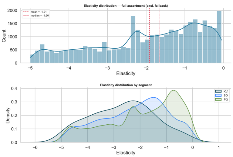
Figure 7. Illustrative elasticity output from a real retail assortment, anonymized. The top panel shows the overall distribution of fitted elasticities. The spread reflects meaningful variation in price sensitivity across tens of thousands of products. The bottom panel breaks that distribution down by commercial segment. KVI (Key Value Items), SD (Sales Drivers), and PG (Profit Generators) products show meaningfully different elasticity profiles.
Elasticity patterns across categories and segments
Different product categories attract customers with very different price sensitivity. A shopper buying a staple food item will respond differently to a price change than someone considering a discretionary toy or accessory. Commercial segment adds another layer: products designated as key value items, sales drivers, or profit generators typically carry different elasticity profiles even within the same category, reflecting their distinct commercial roles and customer expectations.
The table below shows that distinction concretely, drawn from a live retail assortment, with consistent and commercially interpretable patterns across both dimensions. What makes the patterns meaningful is that segment labels are never used as model features. For products with sufficient history, the elasticity estimate is driven by observed price and sales patterns. For sparse-history products assigned to groups via propagation, segment informs the group assignment, but it is never used as a model feature. So when the results still line up with known commercial roles, that is a useful sign the methodology produces interpretable output rather than arbitrary curve fits.
Mean Elasticity by Category and Commercial Segment
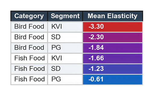
Figure 8. Mean fitted elasticity by product category and commercial segment, drawn from a live retail assortment. The data is real; certain identifying details have been modified to avoid exposing commercially sensitive information. Each row represents a category-segment combination. In practice, the methodology groups products using richer signals than segment alone (price tier, sales history, and other product attributes all contribute to group assignment), but those dimensions are not shown here, both to keep the visualization readable and to avoid exposing proprietary grouping logic. Segment labels (KVI: Key Value Items, SD: Sales Drivers, PG: Profit Generators) are used for group matching and are not used as model features. The color scale runs from blue (less elastic, closer to zero) to red (more elastic, more strongly negative).
Conclusion
Elasticity remains one of the most important tools in pricing, but its value depends on how it is operationalized. A useful methodology must do more than estimate demand response in principle. It must work at scale, hold up against noisy retail reality, and communicate uncertainty responsibly.
A two-stage methodology meets that standard by first expanding the usable demand signal and then fitting a demand model that supports optimization. That combination helps pricing teams move from intuition alone toward more structured, data-informed decisions.
That is the promise of modern elasticity: not perfect foresight, but better commercial judgment.
FAQ
What is price elasticity of demand?
Price elasticity of demand measures how the quantity demanded changes in response to a change in price. It helps pricing teams understand which products can absorb price increases, which require competitive pricing, and where pricing decisions can improve revenue or margin.
How is price elasticity of demand measured?
Price elasticity of demand is measured by comparing the percentage change in demand to the percentage change in price. In retail, however, reliable measurement therefore requires accounting for promotions, seasonality, stock availability, and competitor activity, so that the estimated elasticity reflects price response rather than surrounding market conditions.
What factors affect price elasticity of demand?
While price is a key driver of demand, real-world retail data is influenced by promotions, seasonality, stock availability, competitor pricing, product lifecycle changes, and other commercial factors. These variables must be considered to isolate the true effect of price on demand.
Why is price elasticity difficult to measure in retail?
Retail demand rarely changes because of price alone. Multiple commercial factors often influence sales simultaneously, making it difficult to distinguish genuine price sensitivity from external market conditions. This is why modern pricing methodologies use predictive models to separate meaningful price signals from data noise.
What is the relationship between a demand curve and price elasticity?
A demand curve shows how demand is expected to change across different price points. Price elasticity measures the sensitivity of demand at a specific reference price on that curve, helping pricing teams evaluate the expected impact of different pricing decisions on revenue and margin.
How can retailers use price elasticity to make better pricing decisions?
Retailers can use price elasticity to identify products that can support price increases, protect demand for highly price-sensitive items, optimize promotions, and determine where pricing decisions can be automated or should receive human review.